Before we begin: I have never done any Machine Learning in the past. I am a web developer who graduated with a degree in Economics about 8 years ago. In my Economics classes, I did a bit of regression and at the time I remember it making sense to me after many headaches and hours spent getting my head around it. In the 8 years since, however, I have never needed or used any of this in my day-to-day life and the things I learned have faded into the shadowy depths of my memory.
I’m calling this “Machine Learning Fundamentals” mainly because I have no idea where the things I’m going to be learning fall in the scale of the subject as a whole. Machine learning sounds cool and it seems to be picking up a lot of traction in a range of areas where its potential is being realised.
I am doing the Machine Learning course on Coursera taught by Andrew Ng – to anyone interested in this subject I would highly recommend doing the same. Because the rate of learning is (in my opinion) pretty intense I thought it would be good to help me understand things better by sharing what I learn. Each week, I will try to summarise what I have learned in my own words (hopefully with enough detail to make it a coherent learning tool in its own right), and based on my own understanding – which I suspect leaves a great deal of room for error. Provided that you proceed with caution and a pinch of scepticism my hope is that we will both learn something useful along the way.
On a side note: There will be some material (such as matrices) which will require me to do some outside learning – I won’t cover any of these topics to save those who already have a grasp on them (and save myself a bit of time). I will however share any outside learning material that I find useful along the way.
So there you go, I invite you to come along on this 12-week journey with me and see where we end up. Still reading? Cool.
What is Machine Learning?
I’ll lean on Wikipedia here for a definition of machine learning as it seems fairly succinct:
“Machine learning is a field of artificial intelligence that uses statistical techniques to give computer systems the ability to “learn” from data, without being explicitly programmed”
Okay, let's start off with a simple linear regression case to get our head around some of the techniques we will be applying.
Linear Regression
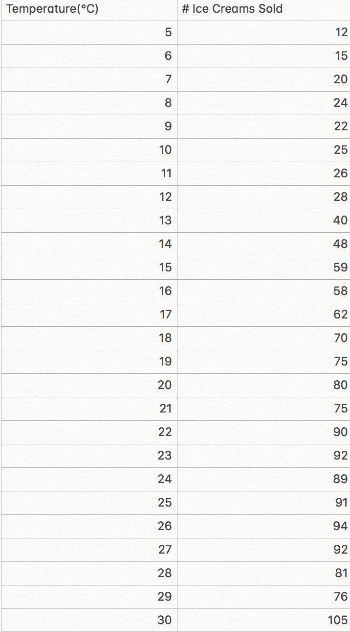
So here is a simple dataset where we are comparing the temperature with the number of ice creams sold.
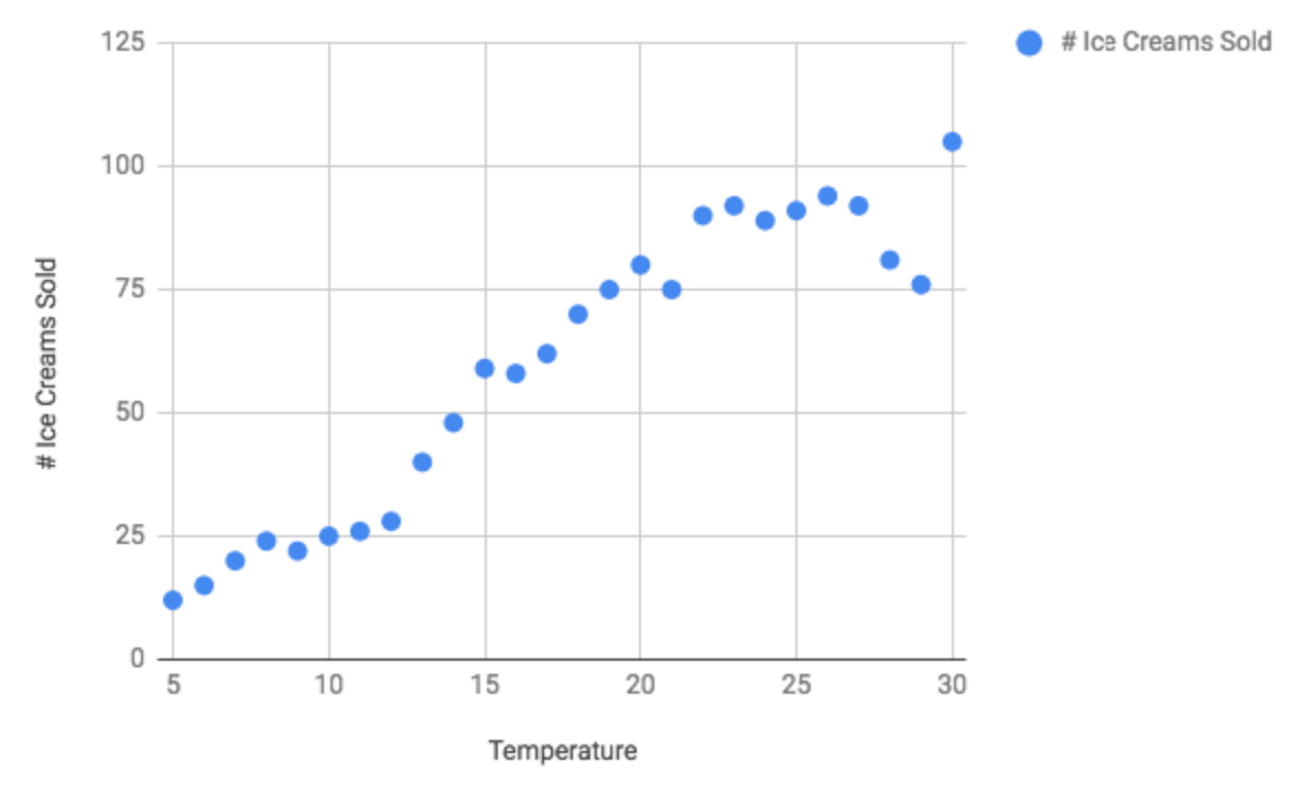
This can be represented by plotting the data on the following graph.
Now let's say we wanted to predict the number of ice cream sales given the temperature on a given day. To do this we could simply plot a line that best fits our data and look at the corresponding point on the line to give us a fairly good estimate.
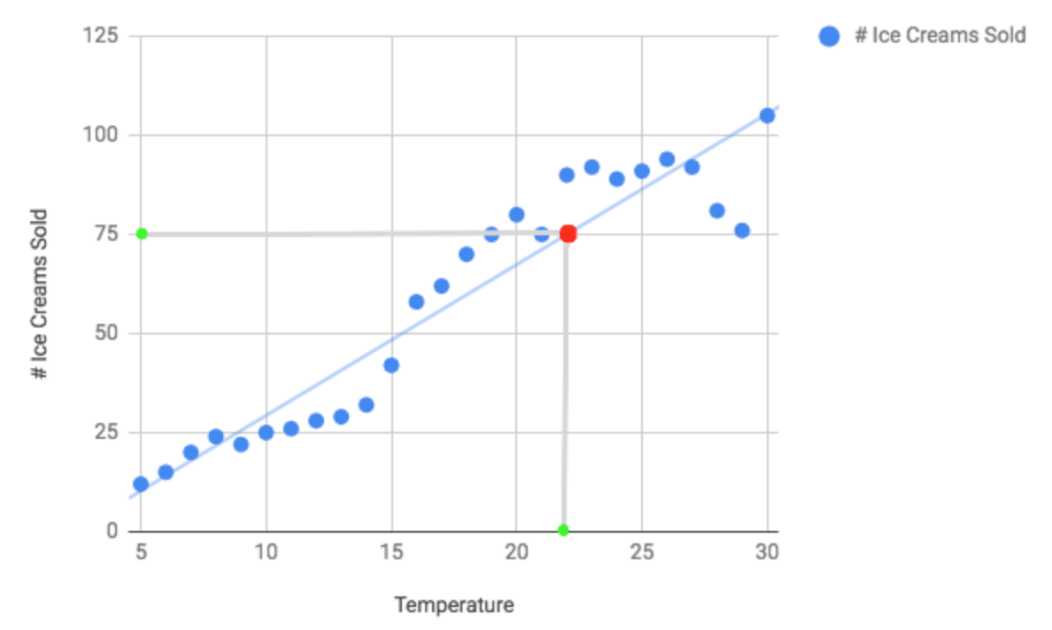
So in the above example, you can see, that with a temperature of around 22(degrees) you would expect to sell approximately 75 ice creams. So how do we work out this line of best fit?
Line of Best Fit
So let's say our line of best fit can be represented by a function of x ( note the use of ‘h’ here as in machine learning this equation is often referred to as a hypothesis ):
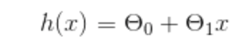
Where ϴ(zero) is a number representing the intersect on the y-axis and ϴ(one) is the coefficient of X ( which will determine the slope of the line ).
So how do we work out the values for ϴ(zero) and ϴ(one)? When trying to plot a line to best represent our data, what we are trying to do is minimise the distances between the actual data points and the line ( the value on the line corresponding to that point ).
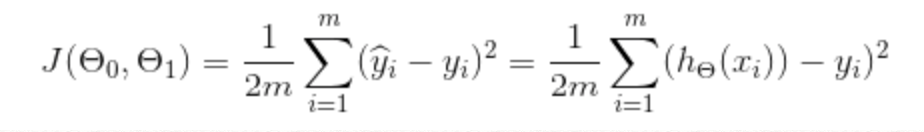
More specifically – we are trying to minimise the sum of the squared differences. ( Squared to weight greater differences more heavily than smaller differences ). Taking this into account what we are trying to minimise can be represented by the following function J( ϴ(zero), ϴ(one) ):
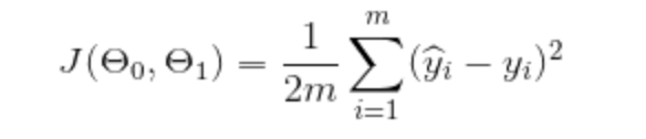
So, what were are doing here is, for each row of our data, taking the difference between the predicted value (Y hat i), and subtracting the actual value (Y i) to get the difference, squaring it and then multiplying this by 1/2m – which is the equivalent of dividing it by 2m, where 2m is twice the number of rows (or observations) in our data. And as we know that the predicted value (Y hat i) will be determined using our hypothesis function we can substitute our hypothesis into the cost function like so:
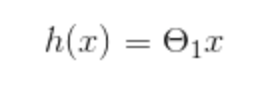
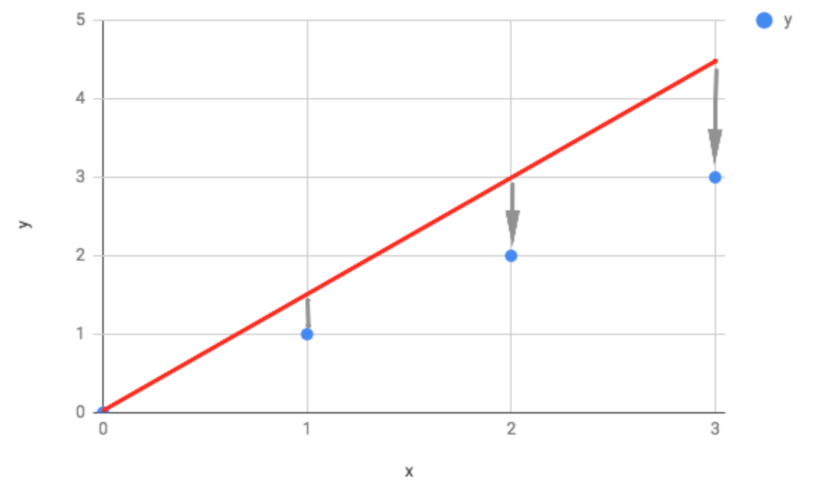
To get a better grasp on the logic behind what's going on here let's look at a simplified hypothesis – where we don’t have the constant (intercept) value.
Okay, so we know the cost function gives us half the average of the sum of squared errors – which is telling us how well our hypothesis fits our data. So with a simplified hypothesis, let's look at what happens to the value of our cost function J for different values of ϴ.
So given a very basic set of data, let's look at what happens when ϴ = 0.5:
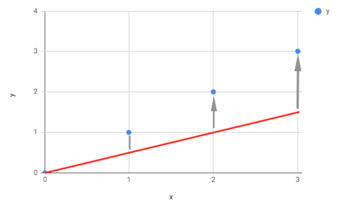
Here you can see the slope of the line is too shallow by the differences between our actual data values and our predicted values ( the line ). Plugging this into our data gives us a value of -0.58 for J(ϴ) when ϴ = 0.5.
How about if ϴ = 1.5:
Here you can see the slope of the line is too steep. Plugging this into our data gives us a value of 0.58 for J(ϴ) when ϴ = 1.5. And if ϴ = 1:
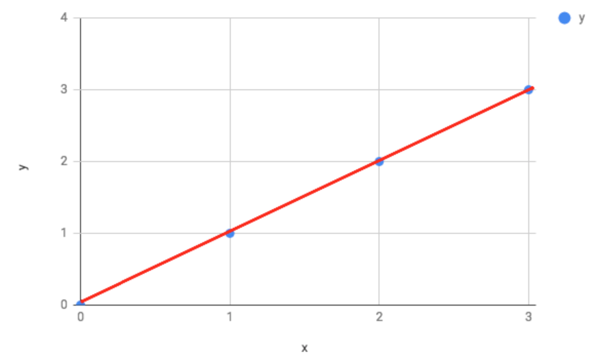
In this case, you can see there is no difference between the actual and predicted values – meaning our cost function will equate to zero.
When the value of ϴ increases, so too does the slope of the line. (Note that without an intercept the line will always pivot about the point (zero, zero)). Given the values determined above, we are able to plot the cost function for different values of theta(one) as shown below.
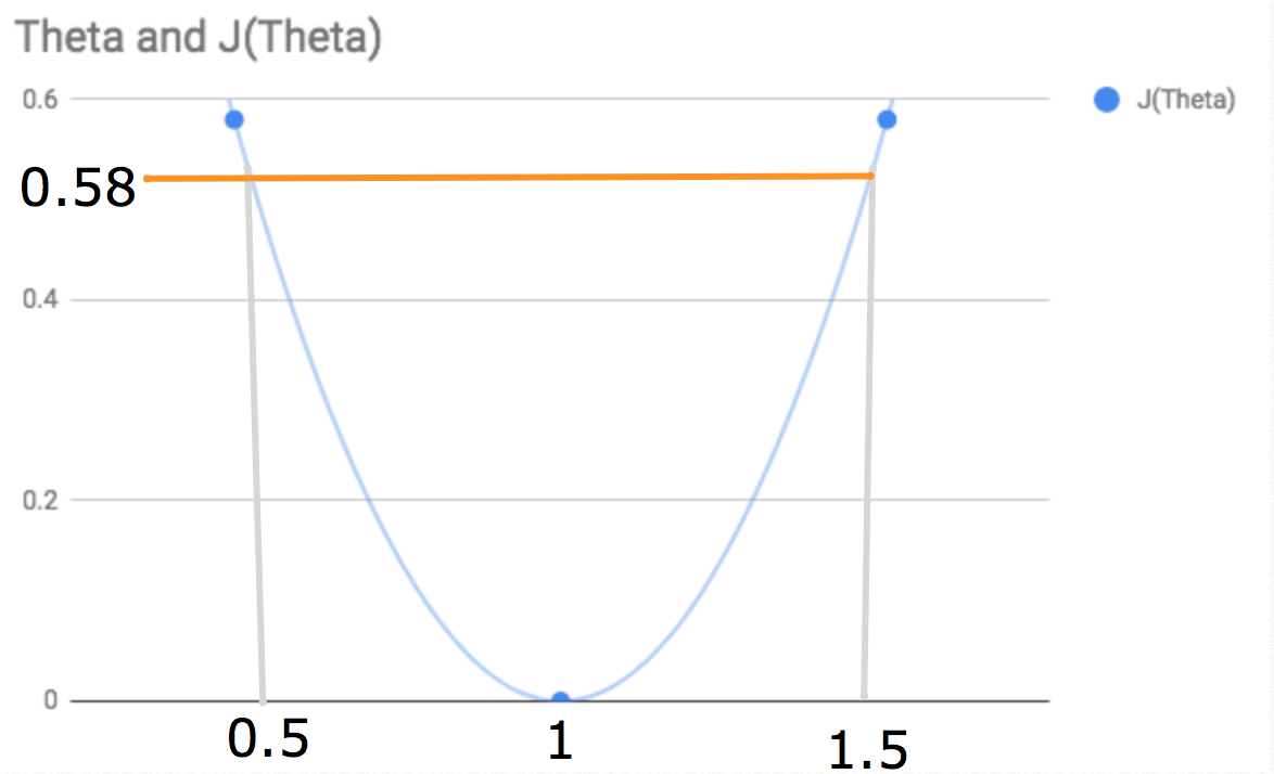
This visually represents the minimal cost for all values of ϴ(one) (the value we are trying to obtain) and we can see that this is 1.
In practice, we are unlikely to be dealing with such straightforward data on such a small scale. You can imagine calculating the above graphical depiction for every given value of ϴ(one) where it could theoretically take any positive or negative value imaginable would be very inefficient.
Gradient Descent
There are a number of ways to calculate this value but the one we will look at here is the method of Gradient Descent. This is a method used widely in machine learning as its application scales well to very large data sets.
When I read the word gradient descent, I picture it translating as “Going downhill” – which luckily is a fairly accurate depiction of what it actually does. The gradient descent algorithm basically takes any given point on the cost function and from that point tries to move downwards in increments until the minimum value for J(ϴ(one)) is attained.
The gradient descent algorithm (for our single parameter hypothesis) is shown below:
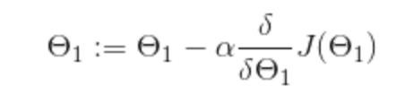
To explain what is happening here, we get a given value for ϴ(one). Then we are looking at the slope of the line at that current point given by the (delta/delta times ϴ(one). We multiply this by some value (alpha) and deduct this from our current ϴ(one) position, update ϴ(one) and do the whole thing again – repeating until the optimum value is found. This is summarised fairly intuitively in the chart for the cost function below – with each incremental step being represented by a red dot.
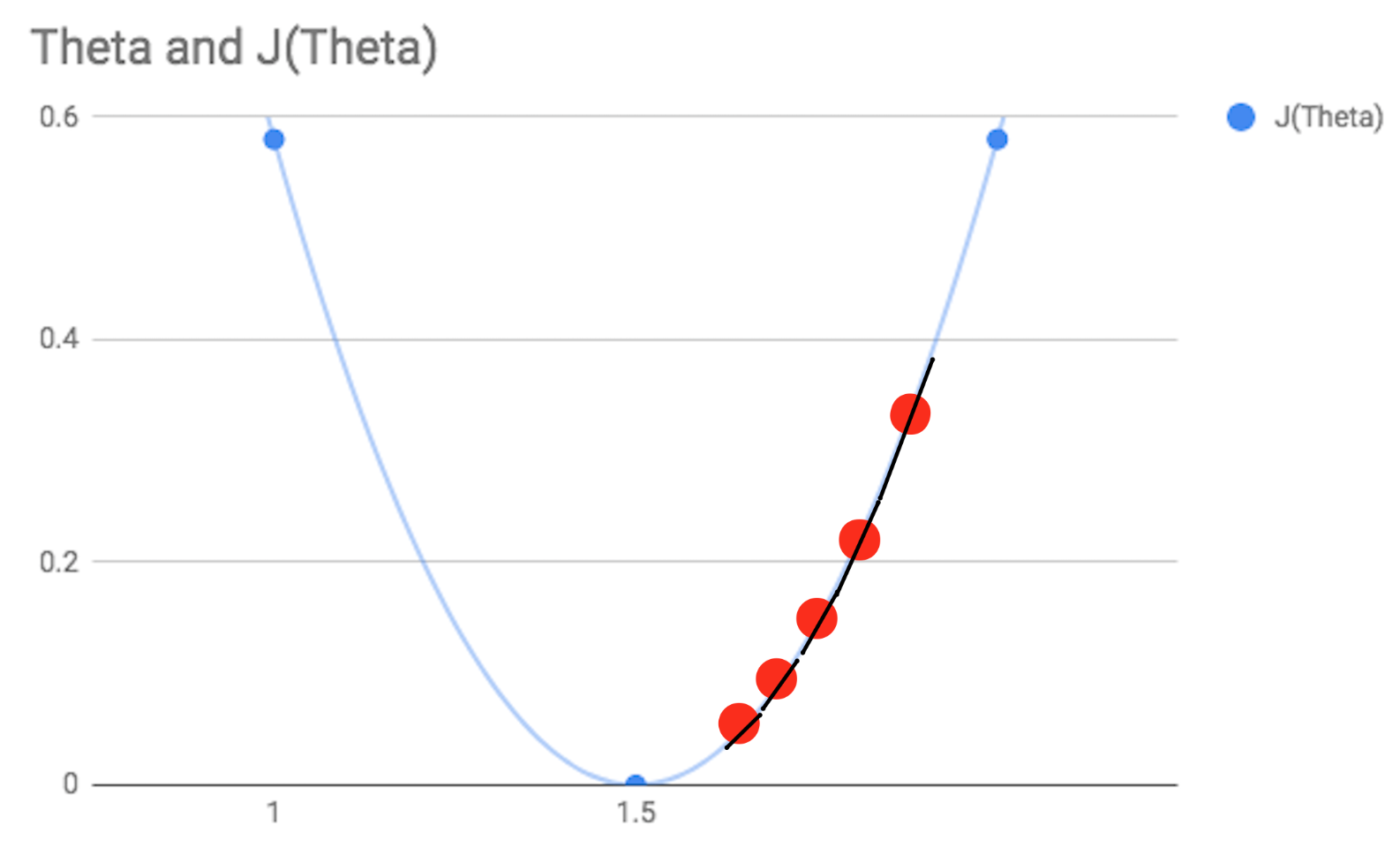
The problem here is we aren’t given a value for alpha, and this value determines the size of the steps we take each time. The way to work out a suitable value for alpha will be discussed in a later post, but for now, it is important to be aware of the issues that can arise from incorrect alpha values.
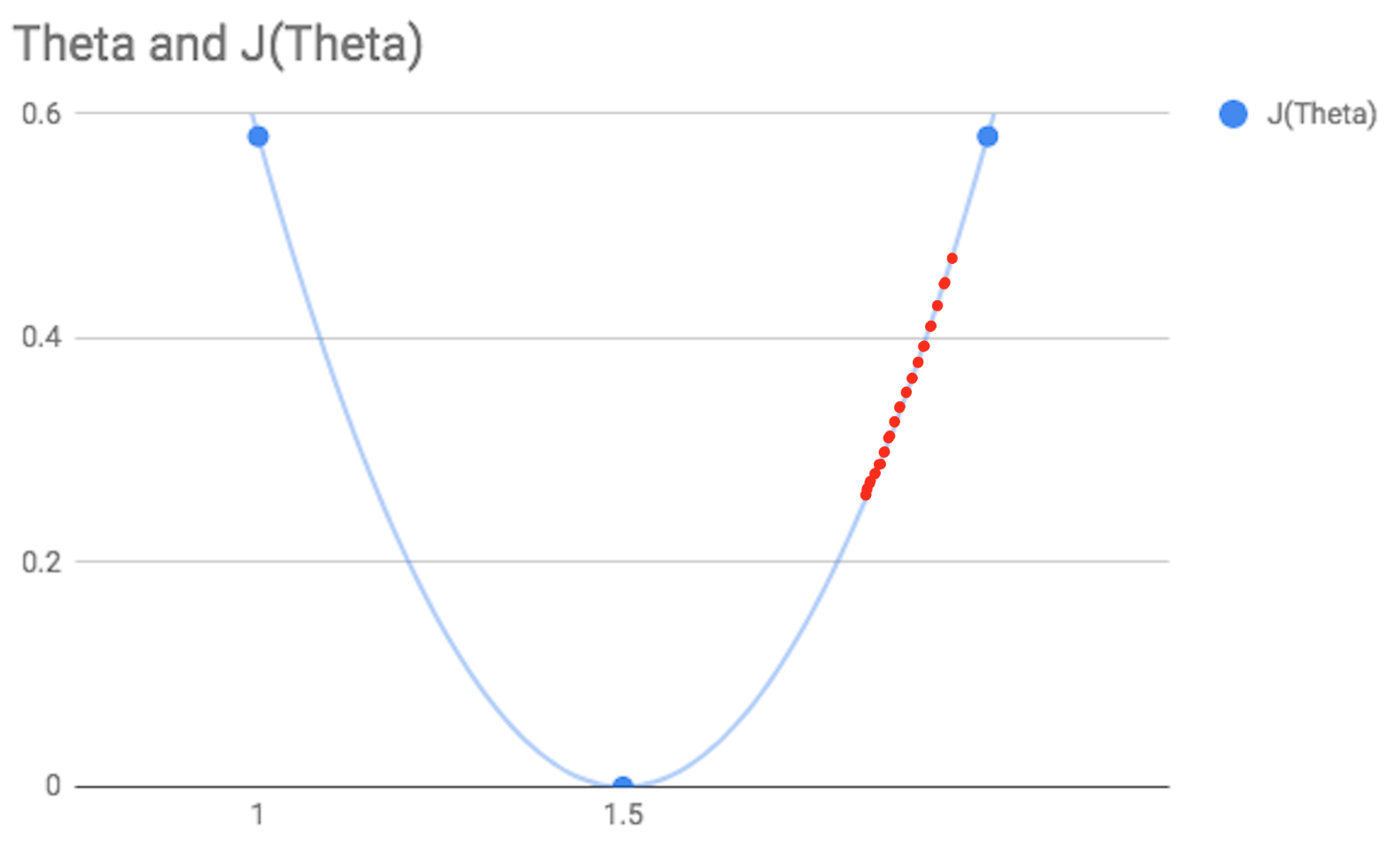
As shown in the diagram below, an alpha value which is too low means that each step taken will be very small and the gradient descent may take a very long time to converge towards the minimum point.
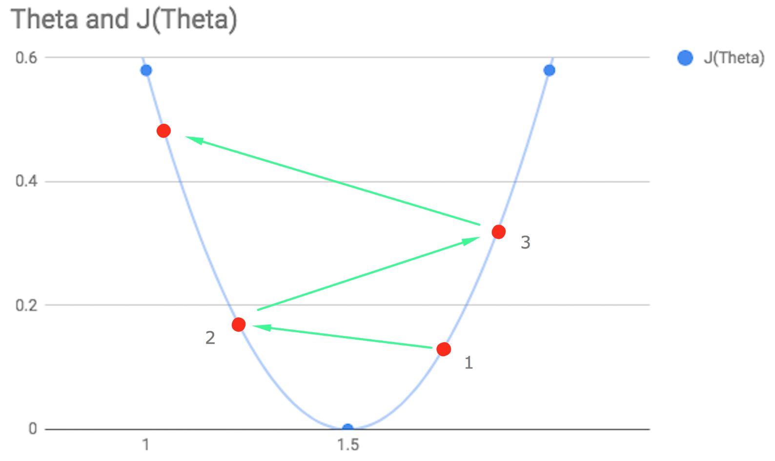
More worryingly (as far as I can tell), an alpha value which is too large may actually cause the steps to be so big that the updated point jumps all the way to the other side of the arch. Given this new value, the gradient descent will then jump an even greater distance in the opposite direction and end up higher still on the opposite side. In this case, instead of heading towards convergence, the updated values from theta one will increase perpetually and no minimum will ever be reached.
If your alpha value is appropriate, however, by its very nature it will take larger steps at further distances from the optimal taking smaller steps as it approaches the minimum. Ultimately landing on an accurate minimum value. As shown in the first chart above.
As mentioned earlier, Gradient Descent provides an excellent approach for determining the optimal values for parameters in linear regression and its benefits tend to surpass alternatives as the scale of the data increases. We will look at ways to determine appropriate alpha values further down the line, but it’s good to be aware of some of the benefits and potential issues when using this method.
Okay, that seems like more than enough to get our heads around for this week. Next time I will explain another way of visualising gradient descent convergence and move on to looking at the use of matrices and vectors to represent data and the benefits of using these when finding the optimal values for theta.